Notes of Graph Neural Networks (Part 02)

1. Introduction

Series are objects playing important roles in the study of calculus. Among the common series, we often especially concern two main sets of series, Taylor ones and Fourier ones. However, I want to use today’s post for Taylor series first because of their capability of extending the definition of some mathematical operations, for example exponential and logarithmic functions. This extension relates to the article I mentioned in the previous post, therefore Taylor series is one of necessary parts to understand the mathematic basis used in the article. Regarding Fourier series, it is a rather complicated topic, therefore I will talk about it in later posts.

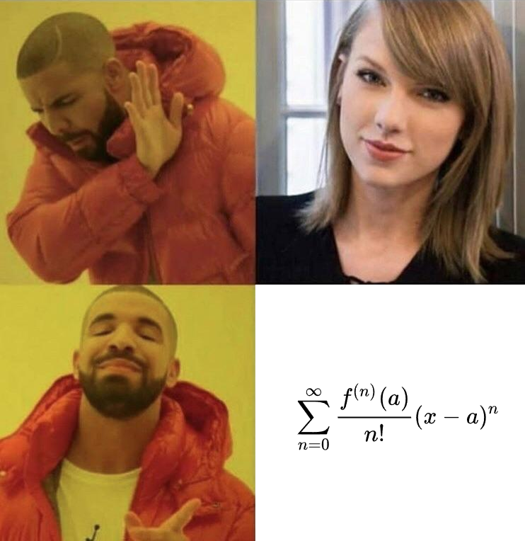
However, please note that this post is completely not relevant to Taylor Swift, except the meme in Figure 1. LOL 🤣

Figure 1. Taylor Swift vs Taylor series.

2. Definition

Definition 2.1. [Ref.] The Taylor series of a function $f(x)$ that is infinitely differentiable at $a$ is the following series

\[f(a) + \frac{f'(a)}{1!}(x - a) + \frac{f''(a)}{2!}(x - a)^2 + \cdots = \sum_{n=0}^\infty \frac{f^{(n)}(a)}{n!} (x - a)^n\]

From Definition 2.1., there are several points we can draw from:

• The condition of constructing Taylor series is the infinitely differentiability. Thus, functions which possess only derivatives of low orders such as $|x^3|$ cannot be used to form Taylor series.
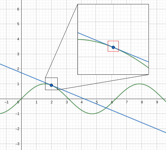
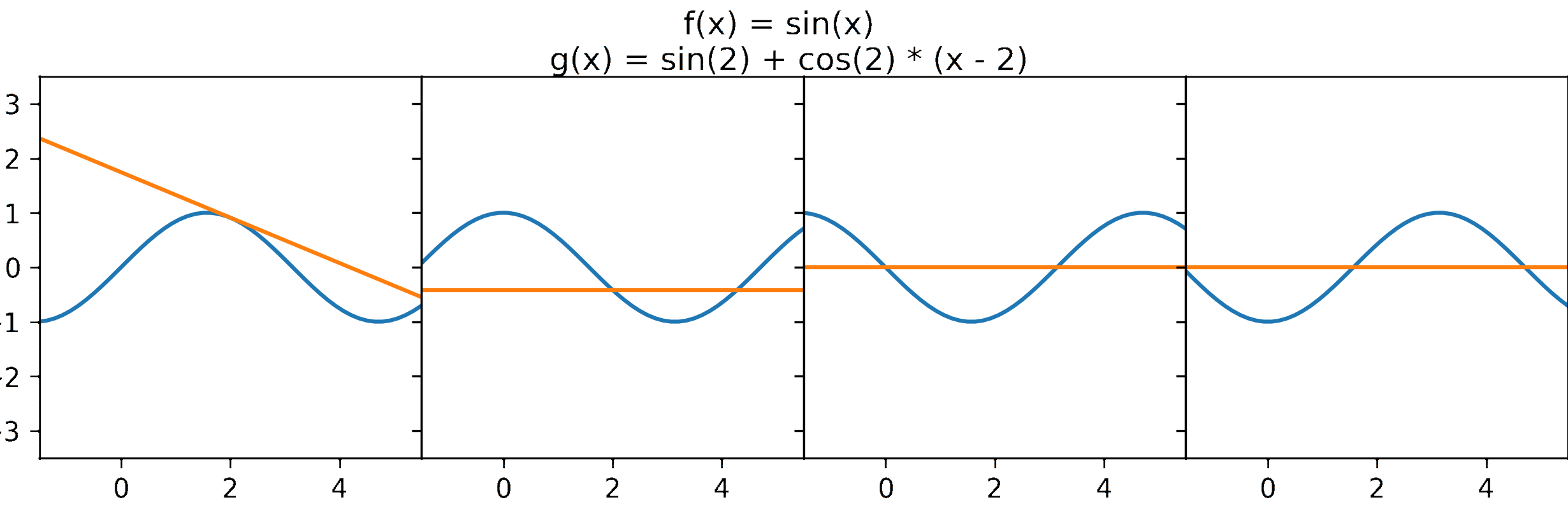
• The sum formed by the first two terms of a Taylor series is also know as the equation of the tangent line. Considering the neighbourhood of $a$, the function $f(x)$ and its tangent line are approximately the same (see Figure 2). This suggests a way to approximate a function. More specifically, if we transform the shape of the tangent line into a curved form, we can achieve a better approximation. It is noted that shape of a function is defined by its derivative. Therefore, to obtain better shape, we need to approximate the derivative, and if we treat it as a function, we can applied the same strategy of using the equation of the tangent line to do that. From that, we infer that the approximate curve is the sum of the first three terms of the Taylor series. Repeating above steps infinitely, we acquire the Taylor series (for illustration see Figure 3).

Figure 2. The function $f(x) = \sin{x}$ and its tangent line $g(x) = \sin{2} + (x - 2)\cos{2}$. In the red square, there are no significant differences between $f(x)$ and $g(x)$.

Figure 3. The function $f(x) = \sin{x}$ and its Taylor polynomials $g(x)$. From left to right are the functions $f(x)$ and $g(x)$, their first derivatives, their second derivatives, and their third derivatives respectively.

So, we can use a Taylor series as an approximate of a function. Even it seems that a Taylor series is exactly equal to the function it represents. However, is this conjecture always true? Can it be false? When is it true, and when is it false? In the next section, I talk about these questions in more detail through a concept called convergence.

3. Convergence of Taylor series

In this section, I only focus the results I consider important. If you want more, you can take a look at other contents here.

For convenience of measuring the approximation, first of all, I need to define several related objects:

• $T_n(x) = \sum_{k = 0}^n \frac{f^{(k)} (a)}{k!} (x - a)^k$ is called the $k$th-degree Taylor polynomial.
• $R_n(x) = f(x) - T_n(x)$ is called the remainder of $T_n(x)$ for $f(x)$.

Because $f(x)$ is continuous at $a$, we obviously have $\lim_{x \to a} R_n(x) = 0$. However, it is difficult to infer anything more useful if the remainder has only this property. Therefore, we need to survey more advanced properties through following forms of the remainder.

3.1. Peano form of the remainder

The idea of this form is derived from the following result:

\[\begin{aligned} \lim_{x \to a} \frac{R_n(x)}{x - a} &= \lim_{x \to a} \frac{f(x) - T_n(x)}{x - a} \\ &= \lim_{x \to a} \frac{f(x) - f(a)}{x - a} - f'(a) \\ &= 0 \\ \end{aligned}\]

This implies that the conjecture $\lim_{x \to a} \frac{R_n(x)}{(x - a)^n} = 0$ can be true. From that, we have the Peano form described as follows:

Peano form: $R_n(x) = h_n(x) (x - a)^n$ where $\lim_{x \to a} h_n(x) = 0$.

One simple proof is using L’Hôpital’s rule as mentioned here. So, I’ll skip the proof of this form and move to the next.

3.2. Mean-value forms of the remainder

Although the Peano form is quite beautiful and simple, it has a significant drawback that we cannot know exactly and specifically what the function $h_n(x)$ is, thus we don’t know too much about $R_n$. Therefore, in this subsection, I will introduce the forms providing more information about this function.

Lagrange form: $R_n(x) = \frac{f^{(n + 1)}(\xi_L)}{(n+1)!} (x - a)^{n + 1}$ for some real number $\xi_L$ between $a$ and $x$.

Cauchy form: $R_n(x) = \frac{f^{(n + 1)}(\xi_C)}{n!} (x - \xi_C)^n (x - a)$ for some real number $\xi_C$ between $a$ and $x$.

You can find the proofs of two above forms here. These proofs use the Cauchy’s mean value theorem. This is an interesting theorem and it’s very useful in some problems. For example, by using the Cauchy’s mean value theorem and the monotonic property of $\frac{1}{x}$, you can prove that:

\[\sum_{i = 1}^n \frac{1}{n} > \ln(n + 1)\]

Therefore, we can infer that the series $\sum_{i = 1}^n \frac{1}{n}$ is divergent.

Hint

Using the Cauchy's mean value theorem, we have: $$\frac{1}{k} > \ln(k + 1) - \ln(k) = \frac{1}{c_k} > \frac{1}{k + 1}$$

We can even prove a better result: $\sum_{i = 1}^n \frac{1}{n} = \Theta(\ln(n))$ where $\Theta$ is the Big Theta notation in computational complexity theory.

Coming back to Taylor series, because these forms use some real numbers between $a$ and $x$, they are called mean-value forms, just like Lagrange’s and Cauchy’s mean value theorems.

3.3. Integral form of the remainder

Another explicit form is also beautiful without using an unknown real number like Lagrange and Cauchy forms or using an unknown function like Peano form. However, to evaluate this form, we need to use integrals, so this form is called integral form.

Integral form: $R_n(x) = \int_a^x \frac{f^{(n+1)}(t)}{n!} (x - t)^n dt$.

The proof for this form can be found here by using induction.

So, we have known some forms of the remainder. These forms help us somewhat guess what will happen when $n$ goes to infinity. More importantly, based on them, we can answer the questions mentioned at the beginning of the post:

• What set does $x$ belong to so that $T_n(x)$ converges?
• Does the limit of $T_n(x)$ equal $f(x)$ when $T_n(x)$ converges?

In the next section, we will find out it.

3.4. Remarks about the convergence of Taylor series

From the Lagrange form, we have:

\[R_n(x) = \frac{f^{(n + 1)}(\xi_L)}{(n+1)!} (x - a)^{n + 1}\]

With some $r > 0$, we assume that $\left\lvert f^{(n)}(t) \right\rvert < M, \forall n \in \mathbb{N}, x \in (a - r, a + r)$, which means $\left\lvert f^{(n)}(t) \right\rvert$ is bounded.

Then, we have:

\[\left\lvert R_n(x) \right\rvert < M \frac{\lvert x - a \rvert^{n + 1}}{(n+1)!} < M \frac{r^{n + 1}}{(n+1)!}\]

From that, we can infer that:

\[\lim_{n \to +\infty} \left\lvert R_n(x) \right\rvert = 0\]

From here, we have several very interesting results:

• $e^x = \sum_{n=0}^\infty \frac{x^n}{n!}, \forall x \in \mathbb{R}$.
• $\sin x = \sum_{n=0}^\infty \frac{(-1)^n}{(2n+1)!} x^{2n+1}, \forall x \in \mathbb{R}$.
• $\cos x = \sum_{n=0}^\infty \frac{(-1)^n}{(2n)!} x^{2n}, \forall x \in \mathbb{R}$.

That means we can consider exponential and trigonometric functions as polynomials of infinite degrees. Then, based on these results, we can extend the definition of some functions (for example, complex numbers). We will discuss in more detail this in the next section.

Besides, we don’t need the requirement that $\left\lvert f^{(n)}(t) \right\rvert$ is bounded to prove that the Taylor series $T_n(x)$ of the function $f(x)$ converges to $f(x)$. For example, considering the geometric series $T_n(x) = \sum_{n=0}^\infty x^n$ which is the Taylor series of $f(x) = \frac{1}{1-x}$, we can see that $\left\lvert f^{(n)}(t) \right\rvert$ isn’t bounded, but $T_n(x)$ still converges for all $x \in (-1, 1)$. If you want to know more about convergence tests, you can read here.

4. Applications

Because of the limit of my knowledge, in this section, I will only present some applications of Taylor series I’m interested most, although there may be still other applications I don’t know. If I have chances to know them in the future, I will present in other posts.

4.1. Exponentiation of complex numbers

To start this subsection, I will introduce you to one of the most beautiful equalities of mathematics:

Euler’s identity: $e^{i \pi} + 1 = 0$.

This equality shows us the relationship between five fundamental mathematical constants, including the number $0$ (the additive identity), the number $1$ (the multiplicative identity), the number $\pi$, the number $e$, and the number $i$ (the imaginary unit). However, it’s very simple and easy to remember, but have you ever wonder why it is like that? If you notice more deeply, you will find out that to understand this equality, we need to define what the exponentiation of a complex number is because of the appearance of the imaginary unit $i$ in the exponent part.

Coming back to Taylor series, we know that $e^x = T(x) = \sum_{n=0}^\infty \frac{x^n}{n!}, \forall x \in \mathbb{R}$. Therefore, if the Taylor series $T(x)$ also converges for all complex numbers $z$, we can use this limit of $T(x)$ to define the complex exponential function.

Considering an arbitrary complex number $z = a + bi$, we have:

\[\begin{aligned} T(a + bi) &= \sum_{n=0}^\infty \frac{(a + bi)^n}{n!} \\ &= \sum_{n=0}^\infty \frac{1}{n!} \left(\sum_{k=0}^n {n \choose k} a^k (bi)^{n - k} \right) \\ &= \sum_{n=0}^\infty \sum_{k=0}^n \frac{a^k}{k!} \cdot \frac{(bi)^{n - k}}{(n - k)!} \\ &= \left(\sum_{n=0}^\infty \frac{a^n}{n!}\right) \cdot \left(\sum_{n=0}^\infty \frac{(bi)^n}{n!}\right) \\ &= e^a \cdot \left( \left(\sum_{n=0}^\infty \frac{(-1)^n}{(2n)!} b^{2n}\right) + i \cdot \left(\sum_{n=0}^\infty \frac{(-1)^n}{(2n+1)!} b^{2n+1}\right) \right) \\ &= e^a \cdot \left(\cos b + i \cdot \sin b\right) \\ \end{aligned}\]

Because $T(a + bi)$ converges, we define

\[\begin{aligned} e^z &= e^{a + bi} \\ &= T(a + bi) \\ &= e^a \cdot \left(\cos b + i \cdot \sin b\right) \\ \end{aligned}\]

where $z = a + bi$ is a complex number.

Of course, the complex exponential function still holds the multiplicative property, which means:

\[\begin{aligned} e^{z_1 + z_2} &= e^{(a_1 + a_2) + i(b_1 + b2)} \\ &= e^{a_1 + a_2} \cdot \left(\cos (b_1 + b_2) + i \cdot \sin (b_1 + b_2)\right) \\ &= \left(e^{a_1} \cdot \left(\cos b_1 + i \cdot \sin b_1\right)\right) \cdot \left(e^{a_2} \cdot \left(\cos b_2 + i \cdot \sin b_2\right)\right) \\ &= e^{z_1} \cdot e^{z_2} \\ \end{aligned}\]

Therefore, we have $e^{i \pi} = \cos \pi + i \sin \pi = -1$ which is Euler’s identity mentioned at the beginning of this subsection. Next, I will try applying the same way for other mathematical objects, namely matrices.

4.2. Exponentiation of matrices

Given a matrix $M$, to apply the same way in the previous subsection, we need the Taylor series $T(M)$ to converge. Thus, $M$ must be a square matrix. Furthermore, I consider only diagonalizable matrices because calculating Taylor series for non-diagonalizable ones isn’t straightforward.

Considering an arbitrary diagonalizable matrices $M = PDP^{-1}$ with $D = \mathrm{diag}\left(\lambda_1,\lambda_2,\ldots\right)$, we have:

\[\begin{aligned} T(M) &= T\left(PDP^{-1}\right) \\ &= \sum_{n=0}^\infty \frac{\left(PDP^{-1}\right)^n}{n!} \\ &= P \left(\sum_{n=0}^\infty \frac{D^n}{n!}\right) P^{-1} \\ &= P D_e P^{-1} \\ \end{aligned}\]

where $D_e = \mathrm{diag}\left(e^{\lambda_1},e^{\lambda_2},\ldots\right)$.

Therefore, $T(M)$ converges, and we can define $e^M = T(M) = P D_e P^{-1}$. Similiar to the previous subsection, the matrix exponential function also has multiplicative property, but the proof is not as simple as the previous one. One way to prove this property is using Newton’s binomial expansion like the proof of the convergence of Taylor series for complex numbers.

This is the mathematical basis used in the article I mentioned at the beginning of this post. The above is two of many possible applications of Taylor series. If I have more time, I will continue to present them in other posts.

Thank you for reading and have a nice day!